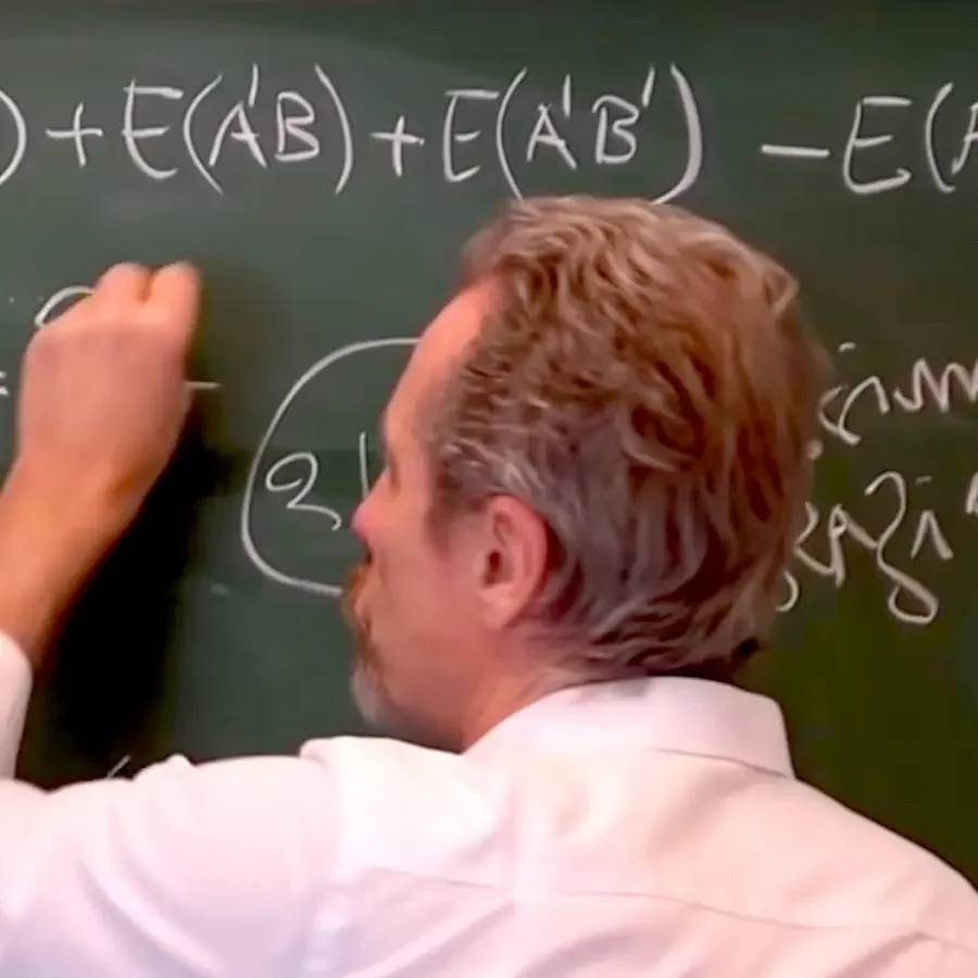
I consider a simple string model (nothing to do with string theory) to explain and (partly) demystify the phenomenon of quantum entanglement. Doing so, I also addresses many objections, presenting at each step a new variant of the model.
The following papers are relevant:
Aerts, D. & Sassoli de Bianchi, M. (2021). Single-entity violation of Bell-CHSH inequality and no-signaling conditions. Journal of Mathematical Physics 62, 092103. https://arxiv.org/abs/1904.06209
Sassoli de Bianchi, M. (2020). Using abstract elastic membranes to learn about quantum measurements. Foundations of Science 25, pp. 77–85. https://arxiv.org/abs/1801.01522
Sassoli de Bianchi, M. (2019). Violation of CHSH inequality and marginal laws in mixed sequential measurements with order effects. Soft Computing (Special Issue on Quantum Structures & Quantum Information Theory). https://arxiv.org/abs/1904.02156
Aerts, D., Aerts Arguëlles, J., Beltran, L., Geriente, S., Sassoli de Bianchi, M., Sozzo, S. & Veloz, T. (2019). Quantum entanglement in physical and cognitive systems: a conceptual analysis and a general representation. European Physical Journal Plus 134: 493. https://link.springer.com/article/10.1140/epjp/i2019-12987-0
Aerts, D. & Sassoli de Bianchi, M. (2019). The Extended Bloch Representation of Quantum Mechanics for Infinite-Dimensional Entities. In: Probing the Meaning of Quantum Mechanics. Information, Contextuality, Relationalism and Entanglement. D. Aerts, M.L. Dalla Chiara, C. de Ronde & D. Krause (eds.) World Scientific, pp. 11-25. https://arxiv.org/abs/1704.06249
Aerts, D., Sassoli de Bianchi, M. & Sozzo, S. (2017). The extended Bloch Representation of Entanglement and Measurement in Quantum Mechanics. Int. J. Theor. Phys. 56: 3727. https://arxiv.org/abs/1609.02658
Aerts, D. & Sassoli de Bianchi, M. (2017). Quantum measurements as weighted symmetry breaking processes: the hidden measurement perspective. International Journal of Quantum Foundations 3, pp. 1-16. https://www.ijqf.org/archives/3777
Aerts, D. & Sassoli de Bianchi, M. (2016). The Extended Bloch Representation of Quantum Mechanics. Explaining Superposition, Interference and Entanglement. J. Math. Phys. 57, 122110. https://arxiv.org/abs/1504.04781
Aerts, D. & Sassoli de Bianchi, M. (2015). Many-Measurements or Many-Worlds? A Dialogue. Found. of Sci. 20, pp. 399-427. https://arxiv.org/abs/1406.0620
Sassoli de Bianchi, M. (2015). God may not play dice, but human observers surely do. Found. of Sci. 20, pp. 77-105. https://arxiv.org/abs/1208.0674
Sassoli de Bianchi, M. (2014). A remark on the role of indeterminism and non-locality in the violation of Bell’s inequality. Annals of Physics 342, pp. 133-142. https://arxiv.org/abs/1302.5826
Is it possible to demystify quantum entanglement?
Well, at least partly demystify quantum entanglement.
Is it possible to explain the mechanism
behind the creation of quantum correlations?
Well, the answer is yes.
Stay tuned.
Entanglement was theoretically discovered
in the 30s of last century by Schrödinger and Einstein.
But then we had to wait the 60s of last century
with the work of John Bell to really have a tool
allowing us to test the presence of entanglement
in physical systems, in experiments.
This tool is the so-called Bell's inequalities.
So the first step to really understand entanglement
is to first acquire the tool of Bell's inequality.
So we will start with that.
Okay, let me briefly explain what Bell's inequalities are about.
I will not explain the original Bell's inequalities
but a version of them called
the Clauser-Horn-Simoni-Holt inequalities.
These are the inequalities
that are actually used in Bell test experiments.
So what is the situation?
The situation is that we have a system, a composite system
and in our case it will be a bipartite system
formed by two parts.
And these two parts are acted upon by two experimenters.
One is named Alice
and the other one is traditionally named Bob.
Okay, now Alice can select among two measurements
she can execute.
One is called measurement A
and the other one measurement A prime.
And these are two outcome measurements.
They can just have two different outcomes.
Same for Bob.
Bob can freely select among two measurements B and B prime.
Now Alice and Bob they perform their measurement jointly,
coincidentally.
Therefore they generate four different kinds of joint measurement.
One joint measurement is AB
where Alice performs A and Bob performs B.
The other one is AB prime
where Alice performs A and Bob performs B prime.
Then of course A prime B and A prime B prime.
Now let us assume that Alice and Bob
they denote the outcomes of their measurement
by using the sign plus or minus.
So they can have either a plus outcome or a minus outcome.
This means that each one of these four experiments
they will have four different possible outcomes.
They can have the outcomes plus plus,
plus minus,
minus plus
or minus minus.
So here Alice has outcome plus and Bob also has outcome plus.
Here Alice has outcome plus and Bob has outcome minus.
Alice minus Bob plus.
And here both Alice and Bob have outcome minus.
So we see here we have two outcomes that we can call them correlated
because the sign is the same.
And here we have two outcomes that are anti-correlated
because the signs are opposite.
Okay so of course now Alice and Bob
they can prepare the system always in the same initial state.
Then they can perform select which measurement to perform each time.
They will do so.
They will collect a lot of data.
And this data will allow them to calculate experimental joint probabilities.
More precisely they will calculate the probability
to have a plus plus outcome for joint measurement A B
or a plus minus outcome for the same joint measurement.
A minus plus outcome or a minus minus outcome.
And of course they will do the same for all these four joint measurements.
So here as well.
So they will collect all these joint probabilities.
Okay so we can collect an entire table of probabilities.
I will not write them all here.
So with all these probabilities for these four joint measurements
they will be able to calculate certain quantities
which are the object of the CHSH inequalities.
So okay let's see how it works.
Well it's not very difficult.
So what we have to do let's consider this measurement.
Let's consider joint measurement A B.
Now to each one of these joint measurements
we want to associate what we will call a correlation function.
Let us denote this correlation function E A B for this joint measurement.
So what is what this correlation function is meant to calculate?
Well we want somehow to quantify how much correlation there is in the system
as opposed to anti-correlation.
Which means we want to quantify in a positive way correlation
and in a negative way anti-correlation
and see what is the trade-off between these two possibilities.
So E A B is simply the following.
We consider the probability for the plus plus outcome
plus the probability for the minus minus outcome.
So we could say that this is the probability for correlation
and then we want to subtract the probability for anti-correlation
which is the probability plus minus plus the probability minus plus.
So you see if we have perfectly correlated outcomes
this first term will be equal to one
and this term with a negative sign will be equal to zero.
So E will be equal to one if we have perfect correlation
and E will be equal to minus one if we have perfect anti-correlation.
And of course E will be by construction
will be in between these two values.
Perfect anti-correlation, perfect correlation
in between a trade-off between these two possibilities.
So these are the quantities that we call correlation function.
And of course for each one of these four joint measurements
we can construct this correlation function.
So we will have four correlation functions that we can use.
Now we will have just to combine this correlation function
I will tell you now how to do so
and this will allow us to state the CHSH inequalities.
Okay, so we have these four correlation functions
that we have calculated from the four different possible joint measurements.
Now we will construct four different quantities.
The first one I will call ACHSH
and this quantity is precisely the following.
It is minus EAB plus EAB prime plus EA prime B plus EA prime B prime.
This is the first quantity.
Then I define, it's really a definition,
I define a second quantity which is exactly the same
but here we have a plus sign and I put the minus sign here.
Then only plus sign here.
Then I define a third quantity where I have the plus sign here,
a plus sign here and now a minus sign here.
So you see I put the minus sign in the different possible places
and of course here I will have a last quantity where I have plus,
plus, plus and the final is a minus.
Okay, so four different possible combinations
where I always combine three plus and one minus.
And now the theorem, the CHSH inequality,
is simply the statement that A or B or C or D,
these four quantities, they have to be bounded
between the values minus two and the values two.
So these are the inequalities to be obeyed.
If these equalities are not obeyed, if they are violated,
then we know that the system was prepared in a state,
in a condition of entanglement.
This is the theorem.
And of course to really explain why this is so,
of course we would have to really derive these inequalities
under a certain number of suitable hypotheses.
I will not do that because this will bring us too far
with respect to the scope of this presentation.
So here we have now the tool and I will use this tool
to study a very simple system.
That's the next step.
Okay, now I want to consider a very simple string model.
A model where Alice and Bob operate on a very simple bipartite system.
This system is simply a string, a white string,
that's right here, it's a white string of length L.
This is the system.
And we can consider it a sort of composite system
because the string has two different ends
on which Alice and Bob can jointly operate.
So they can perform measurement.
Now let me explain what are the measurements they can perform.
So what is measurement A?
Well, measurement A is Alice that measures the length of the string.
And how she does that?
Well, she pulls the string
and then she simply uses whatever instrument to measure its length.
Now, if the length is strictly greater than L over 2,
then the outcome is positive.
If it's not, then the outcome is negative.
So we have plus outcome
if the collected string is longer than half the initial length of the string
or if it's not, then the outcome is minus.
And of course, Bob is exactly the same thing on his side.
Then we have measurement A'.
What is measurement A'?
Well, measurement A' is about the color.
Alice measures the color.
And how she does that?
Well, she simply looks at the string.
If it's white, then the outcome is plus.
And if not white, then the outcome is minus.
And B' for Bob is exactly the same but on his side.
So we have these two different measurements.
One is a length measurement.
The other is a color measurement.
One of the two measurements requires to pull the string.
The other one not.
And Alice and Bob, they perform these measurements together.
Now, what happens when they do so?
Well, here we immediately see something.
When Alice and Bob jointly pull the string...
Now, what I have not told you yet is that the string is breakable.
So if they jointly pull the string, the string will break at some unpredictable point.
Which means that Alice and Bob will just collect a fragment of the initial string.
And of course, depending on the point where the string breaks,
either Alice will collect the longer fragment or Bob.
So you immediately see that they will have anti-correlated outcomes.
And of course, we can neglect the situation where they exactly collect the same length.
Because this is what mathematicians call zero-measure events.
So we see that when Alice performs A and Bob performs B, we have anti-correlation.
On the other hand, when Alice performs A and Bob performs B',
and we assume, of course, they jointly do the experiment in a way
that Bob has enough time to see the color.
Of course, Alice will collect the entire string.
Hence, she will have necessarily a positive outcome.
And Bob will also have a positive outcome because the string is wide.
Which means that the prime experiment, the prime measurement,
they can only have here a plus outcome.
Because, of course, the string will never be observed non-wide.
So in a certain sense, the measurement A' and B' are kind of trivial measurements
with only one outcome.
Okay, so this is the situation.
Now, you immediately see, we don't even need now to calculate the probabilities.
We already know that the correlation function EAB
will quantify a perfect anti-correlation.
So this will be equal to minus one.
Whereas all the other joint measurements,
I forgot the measurement also where Alice and Bob, of course,
they both measure the color.
Of course, they also will get plus plus in this situation.
So all the other joint measurements will have the same correlation function.
And this correlation function will quantify a perfect correlation.
So their value will be equal to one.
Now, at this point, it is easy to calculate these quantities
that are involved in the CHSH inequality, Bell inequality.
And let's consider the quantity we call ACHSH,
which if you remember, it was minus AB plus AB'
plus B' AA'B plus AA'B'.
Now you see, here I have minus one.
Here I have one.
So I have minus minus one.
This is one plus one plus one plus one.
Well, this is four.
And four, no doubt about that, is strictly greater than two.
Hence, we have a violation of Bell CHSH inequality.
OK, before continuing, let me say that this string model
is a variant of an ancient model that was invented
by the Belgian physicist Diederik Aerts.
And at the time, it was called the vessels of water model.
So this is exactly the same model, but now using a string,
so it's a sort of simplified version.
OK, now, are you surprised by this result or not?
Well, maybe you are, maybe you are not.
We have here a very simple physical situation
which manifests a violation of Bell's inequality.
For some physicists, this is quite strange
because in the head of many of my colleagues,
Bell's inequality, Clausenholz-Simoni-Holtz inequality,
they have to do with the micro world,
with the atomic and subatomic world.
And they are not used to think about these inequalities
being violated in the macro world of ordinary object.
So this is possible.
We can have this kind of violation.
Now, what kind of insight can we gain from that?
Well, why do we have a violation?
Well, the reason for that lies in a difference
between correlations of the first kind
and correlation of the second kind,
to use a terminology that was introduced
a long time ago by the etheric arts.
So correlation of the first kind are simply those correlations
that were already actual
before the execution of the joint measurement.
Whereas correlation of the second kind,
these are correlations that prior to the joint measurements
are only potential.
And these correlations are contextually actualized
at each run of the joint measurement.
And here you can really see that
because you see when Alice and Bob pull together the string,
when they perform measurement AB,
they jointly pull the string
and they create a correlation
which was non-existent prior to the measurement.
Because of course, we don't know where the string will break.
At each run of the measurement,
there will be fluctuations which are not possible to control.
And these fluctuations explain the indeterminacy of the outcomes
and also are at the origin of this correlation
of the second kind,
which are created at each run of a joint measurement.
Now, is this the fundamental explanation
behind the violation of Bell's CHSH inequalities?
Well, the answer is yes.
This is the correct way of thinking about these violations.
And now let me show this in very simple terms.
Let us consider the following.
What would happen if instead of a whole string,
Alice and Bob would operate on a string which is already broken?
Imagine Alice and Bob have a friend called David.
David likes to make pranks
and he cuts the string before the execution of the measurement
in some unpredictable point, of course,
but the string is already broken in two parts.
So what changes now if the string is already broken?
Of course, when we consider measurement AB,
nothing really changes.
We will still have that AEAB is equal to minus one.
So the change is not at the level of the joint measurement AB,
nor it is at the level of the joint measurement A'B',
because these are just about the color of the string.
But there will be a difference for the two measurements A'B and B'A.
Why?
Well, because now when Alice pulls the string,
she will not anymore systematically collect the full string of length L,
which means that she will not always have a plus outcome,
but she can also have a minus outcome.
And same for Bob.
When Bob pulls the string,
and Alice just performed the color measurement,
he can only pull a fragment of it,
which can be longer than L over two or not.
So we see that now we have a situation with these two correlation functions
where we have the possibility of correlated outcomes,
but also anti-correlated outcomes.
And this means that this time these two correlation functions
will be equal to zero.
So here I will not have that.
Here I will have zero.
Here we'll have zero.
And now I have minus minus one is one plus one.
Now I don't have four, but I have two.
And two is not strictly greater than two,
hence I don't have anymore a violation.
So you see that the fact that correlations are not anymore of a second kind,
but they are now all of them of the first kind in the model,
because the string is already broken,
then this means that there is no more any violation.
Well, a nice little model indeed.
I mean, it definitely violates the Bell CHSH inequalities.
And yes, I have to admit in the beginning I was thinking
that an error was lurking in there somewhere,
but the calculations are so simple and I could really check them.
There's no error, so indeed it violates these inequalities.
But, but, but, it is also true that it does so with a magnitude of four,
which is the algebraically maximal possible value.
And we know that in quantum mechanics we have a bound called the Chiral zone bound,
which is two square root of two, so 2.8 and something.
And this is really smaller than four.
And so it seems to me that your beautiful little toy model,
it has not a lot to do with quantum mechanics,
precisely because it violates these inequalities too strongly.
Okay, yes, I see.
This is a valid objection.
I imagine that one can be suspicious about a violation,
which is the maximum algebraic possible value.
So let me see if I can modify, slightly modify the model,
so as to have milder violations.
Okay, so in order to address this objection,
let me consider a slight variation of the previous model.
We still have a string, a string of length l,
but now the difference will be that the string can also be blue in color.
It can either be white or blue.
You can think that the material is unstable,
so it switches from blue to white from time to time.
Or you can think that the friend David, before the joint measurement,
sometimes he replaces a white string with a blue one and vice versa.
But let us consider that we know the probabilities of this fluctuation.
Let us assume that Pw is the probability for the string to be observed white,
and Pb the probability to be observed blue.
Apart from that, we are exactly in the same situation as before.
Alice always performs the color measurement a' and the length measurement a',
and Bob always performs as well these two measurements b and b'.
Now, of course, when Alice and Bob jointly perform the a-b joint measurement,
they both pull on the string, they will break it, they will collect anti-correlations.
So here, of course, the correlation function eab will always be equal to minus one.
And also the fact that the string can change color
doesn't change anything about the measurement a'b',
because, of course, even if the string can change color,
Alice and Bob jointly only observe the same color.
So this means that eab' will be equal to plus one.
Now, where there is a difference is, of course, in the two measurements a'b or b'a,
because now when Alice pulls the string to measure its length,
and Bob just observes the color, of course, Alice will collect the entire string.
So she will always have a positive outcome.
But Bob, of course, he can either have a plus or a minus outcome depending on the color.
And here it is the same thing.
So now we have a situation which is a little bit more complex.
And it is very easy to check that in this case,
these two correlation functions now will be given by the probability to be white
minus the probability to be blue.
So now if we calculate the quantity a ch sh, we know that it is minus eab.
So this now is minus minus one.
So it is one.
Then we have these two quantities.
And these two quantities now are twice p white minus p blue.
And the last term, of course, is a'b'.
And this is, of course, one.
So we have one plus one is two plus two p white minus p black, not black, blue.
And p blue, of course, is one minus p white.
So here we have, of course, one minus minus one plus two p white.
So this gives two minus two plus four p white.
So we find that this quantity is equal to four p white.
And of course, if the probability to be white is one,
then we are back to the previous example.
But this probability now, it can be anything from zero to one.
So we really see that we can have all sorts of situation.
We can violate Bell's inequality, the ch sh version with whatever magnitude.
And for instance, if we take p white to be square root of two over two,
then the violations will be exactly equal to two square root of two,
which is so-called the serial zone bound, which is the maximum value in quantum mechanics.
So I think we have now correctly addressed the objection.
The model is complex enough to allow for violation of different order.
Therefore, this is not the problem of this very simple model
in terms of possibly explain quantum correlations.
Interesting.
So the model is also able to violate the inequality in a milder way.
That's good.
I'm impressed.
But I have bad news, because I just discovered that your model
violates also the so-called no-signal conditions.
And these conditions are instead obeyed by quantum systems.
Because quantum systems, the joint measurement are modalized by product measurement.
And so this ensures the obedience to these no-signaling conditions.
So I'm afraid your model does not describe the actual mechanism behind quantum correlations.
OK, it is true that the model violates the so-called no-signaling condition or marginal laws.
But is this a true limitation of the model?
Can we again make it a little bit more complex in order to have a situation
where we have both a violation of the CHSH inequalities
and no violation of the no-signaling conditions or marginal laws?
Well, this is possible.
And this will be the next step.
OK, so now I have to address the issue that the model does not obey the marginal laws,
the so-called no-signaling conditions.
And of course, this is a strong objection,
because in quantum mechanics, we have an obedience to these marginal laws or no-signaling conditions.
Well, at least this is what it is believed.
In experiments, the situation is much less clear,
because apparently these no-signaling conditions are constantly violated in experiments.
But we think this is mostly due to error in experimental errors.
So this is not fundamental violations.
Is it really so?
Well, that's something that needs to be clarified.
But OK, let's for a moment remain with our issue here.
We have a model violating these marginal laws.
And the objection is we need at least a model which obeys them,
to think that this model can somehow explain the origin of the quantum correlation.
So OK, let me do so by slightly now changing again the model.
But before doing so, let me first see with you
what it means exactly to violate these marginal laws.
Otherwise, we don't understand each other.
So let me be back for a moment to the previous model.
So let me give you what are the different joint probabilities,
which I didn't describe before explicitly.
So let me write here p plus plus for the correlation,
p plus minus, p minus plus, and p minus minus.
And now here I have the four possible measurements,
a, b, a, b prime, a prime, b, and a prime, b prime.
OK, these are all the situations.
So now let me construct a table here.
It's not difficult.
This is the table.
So we will have all the possible values.
Now, of course, here we will have one half and one half,
because of course there is equal probability for Alice and Bob
to get the longer fragments.
The string is here assumed to be homogeneous.
And then here we have p white, then we have p black, p blue,
0, 0.
Then we have p white, 0, p blue, 0, p white, 0, 0, p blue.
And I leave it to you to check that these are exactly
the joint probability of the problem we have previously considered.
Now you immediately see here that if I want to calculate
the probability for Alice when she performs measurement a
to have a positive outcome irrespective of the outcome of Bob,
then if Bob is jointly performing measurement b,
when what it will be this probability,
then it is the probability having plus.
So it's that probability plus that probability
with Bob who can have either plus or minus.
So I have to sum this probability with that one.
So it is 0 plus one half, and this is one half.
But I could also consider the situation of Alice
having a positive outcome while measuring a
with Bob executing measurement b prime.
And in this case, of course, I am on this line.
And then, of course, the probability are these two.
So it's p white plus p blue.
And this, of course, is equal to one.
And one is different from one half.
So these marginal probabilities are different,
which means that Alice has somehow the possibility
by analyzing her probability to understand
what kind of measurements Bob is jointly performing.
OK, so this is the violation.
Now I need to show that it is possible to consider
a model where there is no such violation.
So how can I do that?
Well, a possibility is to consider exactly the same situation.
But this time, I will define measurement a and b
in a different way.
Now a and b will be, let's say,
let's consider the situation for Alice.
For Bob, it will be exactly the same thing.
Now Alice, when she performs measurement a,
she will still pull the string and measure its length.
But she will also measure its color.
And she will consider the correlation between length and color.
And so she will consider that if it's long and white
or short and black, this correspond to outcome plus or.
So long white, short black.
She will jointly consider these two properties
and the correlation.
And of course, if it will be short white or long black,
it will be otherwise, it will be the outcome minus.
And Bob will do the same when performing b.
So this changes the experiment, the situation, of course.
I've just changed the measurement that Alice and Bob perform
on their subsystems.
Okay, now one can think about what changes
in terms of the probability, the joint probability.
So I leave it to you to go into the details of a model.
Otherwise, it will become a little bit boring
if I do all this here on the blackboard.
But what is important to see, this you have to believe me somehow,
is that with this new definition of the a and b measurement,
then the probabilities here will change.
And we will now have here 0, 0.
Here we have p blue, p blue, and p blue.
So we have this different table now.
And now you see with this different table,
you see that what happens is that, of course,
for this marginal, it will be the same thing, one half.
But for this marginal now, I have this plus 0.
So instead of that, I have this plus 0.
And this is white.
And now, of course, if p white is exactly equal one half,
which is a choice I can make,
then my model obeys, perfectly obeys the marginal laws.
In this situation, one can check that all the other marginal laws
are obeyed as well.
But now this model, of course, violates the Bell-CHSH inequalities
because we have perfect anti-correlation for this measurement
and perfect correlation for the others,
which means that the quantity a is exactly equal to 4.
So we have, again, a maximal violation of the Bell inequality
and a perfect obedience of the marginal laws.
And this, of course, I think addresses the objection.
Okay, congratulations.
So you managed to have violations of Bell's CHSH inequality
and obedience to the no signaling conditions.
Good.
But the violation now is back to the 4 value.
It's again a fixed value of 4, the maximum value.
So it seems to me that if you try to fix one part of your model,
then another part of it has a problem.
I'm afraid that this model is nice, but not the real deal.
Okay, so now I have to address this, I hope, last objection.
This last objection is, yes,
about the fact that what I have shown you previously
is a situation where indeed you have obedience of the marginal laws
of the no signaling conditions
and a violation which is algebraically maximal.
And now the objection is, well, yes, but again,
this is kind of pathological to have this maximal violation
which is not obtainable in quantum mechanics.
So let me show a situation where we can have
not only the non-violation of the marginal laws,
but also the possibility of having different degrees of violations
of Bell's CHSH inequalities.
All right, so one has to think again how to complexify
a little further the model to have it rich enough
to also be able to describe such a situation.
Now, what I'm gonna do is I'm going to keep
the measurement of Alice and Bob exactly as they were.
So the prime measurement are just about color
and the A and B measurement are about the correlation
between length and color, but it's not enough.
So I will now consider the system as being made now
by two string instead of one.
Two string, which can be white or blue
with these probabilities, of course,
which are the same for the two strings.
Of course, I could consider different probabilities
for the two string, but it become too complicated.
And so I have two string now.
And so Alice, when they pull, they might pull one
or the other, so the system is a bit more complex.
And let's say that they will pull this string
with probability P1 and this one with probability P2.
Let's say that this probability P1 and P2
are the same again for Alice and Bob
because there is no need to make the model too complicated.
Okay, so I have now not only these P white
and P blue probabilities, I have also a probability
of pulling string number one or string number two.
And of course, this will introduce much more structure
in the model because now, as you can imagine,
there is the possibility for Alice and Bob
to jointly pull a long string.
I mean, the entire string, it's sufficient
that they pull a different string
and they now can also have different colors
because of course, again, if they pull a different string,
the color need not anymore to be perfectly correlated.
So you see, you have a much richer combination
of possibilities.
Now, of course, I could try with you
to go into all the details,
but now the calculation become a little bit more involved.
They are not difficult, but you really have to be careful
to take into account all these possibilities.
So now you have really to trust me,
otherwise, again, the video will become just boring.
So I have done properly all the calculation
and now the result of this calculation
is that the correlation function EAB
is minus one plus four P one, P two.
And here in the parentheses,
I have one minus two P white, P blue.
This is the expression.
And for the other correlation function,
they are all the same
and they are given by one minus eight P one,
P two, P white, P blue.
So this is the result.
Now, of course, now you can put this inside
the quantity ACHSH and look what you obtained.
Now, before doing that,
one also has to now check what happens for the marginal law.
So I will not do all this because it becomes huge calculation.
But what I can tell you is, trust me, please,
is that when you set again P white equal P blue equal one half,
then again, as before,
the model perfectly obeys all the marginal laws.
So from that viewpoint, we are safe.
But now if we have this,
we can also show that in this circumstance,
then this A quantity, which is in Bell's inequality,
is equal for P one square plus P two square.
And this you see immediately that this, of course,
it can be equal to four.
If let's say P one equals one or P one equals zero,
of course, then you will have the maximum violation.
But we can also have different degrees of violation, of course.
If, for instance, we have P one equal P two equal one half,
then P one square plus P two square will be one fourth plus one fourth,
which is one half.
And then you see that in this case here,
if P one equal one half,
then we will have four divided by two, which is two.
So we have no violation in this situation.
So we can go from the minimum violation to the maximum one with no problem.
So again, the model has enough richness.
And of course, in between, you can also reach the two square two value,
which is the maximum value for quantum mechanics.
So I have shown now that the model with all this variation
can reach the stage of being able to obey or not obey the marginal laws
and to violate or not violate Bell's inequality.
So we have all this freedom.
And so the mechanism which is behind these violations is general enough.
And it's probably, I would say,
the mechanism which is also behind the violation in quantum experiments,
which is the fact that we have some hidden interactions
when the measuring system interacts with the measured system.
We have interactions which are potential,
you know, as all these breaking points are potential.
And these are actualized every time.
So this model provides a lot of insight into what is a possible mechanism in force.
Also, when we perform experiments on entangled microscopic entities.
Well, I'm impressed.
You succeeded to respond to all my criticism.
Very good.
Bravo, bravo.
But I am still not believing that the mechanism that your model makes explicit
would be the mechanism in force in atomic and subatomic systems.
Because, you see, if this would be true,
I think that these hidden interactions,
which would be responsible for this correlation of the second kind, as you call them,
this should appear somewhere in the quantum formalism,
which I think is not the case.
Okay, yes.
Thanks for this last criticism.
Yes, I understand that one would like to have within the quantum formalism
a hint about the possible existence of these hidden interactions
that would explain how these correlations are each time created
when we execute the joint measurement,
the equivalent of this breaking point of the string.
Now, the good news is that, in fact,
there is a way to represent the states in quantum mechanics
and not only the states, but also the measurement,
which precisely suggests the existence of these hidden measurement interaction,
potential non-local interaction between the measured system and the measuring apparatus.
So this representation is called the extended block representation of quantum mechanics.
It happens inside the so-called block spheres,
a generalization, of course, of the block sphere,
because when you have measurement having more than two outcomes,
the block spheres is not only three-dimensional,
but it can become n squared minus one dimensional,
so everything becomes much more complicated, of course.
But you still have very nice structures inside,
inscribed in the block spheres, which are simplexes,
which represent this potentiality region,
which is at the origin of the creation of correlation of the collapses and so on.
So, actually, there is, within the quantum formalism,
the indication that what is also suggested by this model
would be in force also at the microscopic level.
Of course, nobody up to now has ever directly observed
the existence of these hidden interaction,
and let's hope that in future experiments we'll be able to do so.
Okay, okay, so there is, after all, an indication in the quantum formalism
that these hidden measurement interactions
responsible for this creation of correlations
may exist, even though remaining still at the sub-empirical level for us.
But, yes, let's hope we will be able one day to have evidence of their existence.
And I think that if this will be true, some Nobel Prizes will come indeed.
But let me express a last point of criticism.
When you have two entangled electrons or photons or whatever
which are flying away and they are separated by very large spatial distances,
what would be in this case this connective element
which would play the role of the body of the string, so to say?
Because you can find nothing in between them.
And this, in my view, is a very strong counter-argument
for your model. What do you think?
So, yes, this is where quantum entanglement becomes really mysterious, of course,
and really different from the situation of a macroscopic object-like system like our string.
Of course, the string which Alice and Bob experiment on is a whole entity.
You can consider it as the joining of potential fragments
which can be of different lengths, of course.
And these strings, of course, they are kind of interconnected
through the very body of the string.
So Alice and Bob, they can operate at the two ends
and the string itself plays the role of a connective element.
But now when you have, say, two electrons with their spins
flying away, very far away in space, you cannot find anything within them in space.
So there's nothing in space which you can think about
which would play the role of an interconnective medium
explaining the creation of a correlation.
But it would be wrong to think of these quantum entities
as entities that would be representable entirely within our space-time theatre.
And these connections within the extended block formalis,
they can represent it, formalise,
and we see that they have a dimensionality
which is much higher with respect to the dimensionality
of the individual state of the subsystem.
So there are reasons to believe that these interconnections exist
making the entangled system as a whole
but they are not manifest, not available to be detected
using three-dimensional measuring system.
And here, of course, we touch the true mystery of quantum mechanics
which tells us somehow that our reality is not fully contained
within our spatial-temporal theatre
which is too small to represent all the typologies of entities
that exist out there and their possible interaction.
Thank you for listening.
Okay, hello and thanks for all these very nice explanations.